PluriGaussian - ND truncated Gaussian

Plurigaussian simulation is a type og truncated Gaussian simulation. It works by generating a number of realizations of Gassuan models, each with a sepcific choice of covariance model. Using a transformation map, the Gaussian realizations are then converted into disrete units.

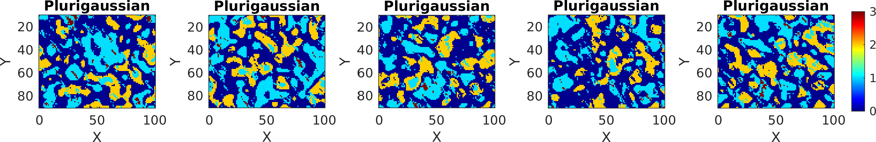
PluriGaussian based on 1 Gaussian

A simple example using 1 Gaussian realization, one must specify one covariance model one plurigaussian transformation map through the two fields prior{1}.pg_prior{1}.Cm(or Cm) and prior{1}.pg_map.

The covariance model is defined as for any other Gaussian based models, and can include anisotropy. In general, the variance (sill) should be 1. Unless set othwerwise, the mean is assumed to be zero.

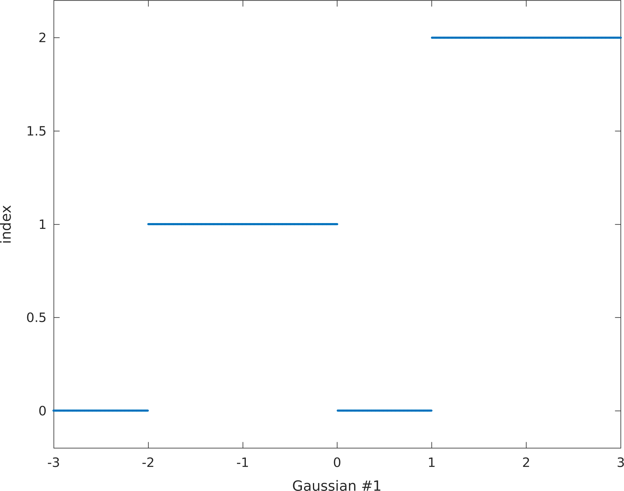
The values in the transformation map is implicitly assumed to define boundaries along a linear scale from -3 to 3. As there are 7 entries (see below) in the transformation map, each number in the transformation map corresponds to [-3,-2,-1,0,1,2,3] respectively. The figure below show what unit id's any Gaussian realized value will be transformed to.

im=im+1;
prior{im}.name='Plurigaussian'; % [optional] specifies name to prior
prior{im}.type='plurigaussian';                % the type of a priori model
prior{im}.x=[0:1:100];                 % specifies the scales of the 1st (X) dimension
prior{im}.y=[10:1:90];                 % specifies the scales of the 2nd (Y) dimension
prior{im}.Cm='1 Gau(10)'; % or next line
prior{im}.pg_prior{1}.Cm=' 1 Gau(10)';
prior{im}.pg_map=[0 0  1 1 0  2 2];
[m,prior]=sippi_prior(prior);          % generate a realization from the prior model
sippi_plot_prior_sample(prior,im,5)
print_mul('prior_example_2d_plurigaussian_1')
figure;
pg_plot(prior{im}.pg_map,prior{im}.pg_limits);
colormap(sippi_colormap);
print_mul('prior_example_2d_plurigaussian_1_pgmap')

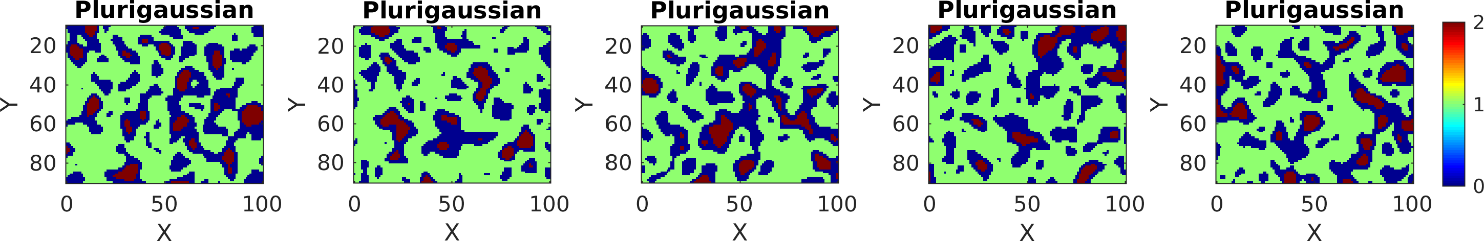
PluriGaussian based on 2 Gaussians

Plurigaussian truncation can be based on more than one Gaussian realization, In the example below, two Gaussian realization are used, and therefore a transformation map needs to be defined. Each dimension of the transformation map corresponds to values of the Gaussian realization between -3 and 3. The transformation maps is visualized below.

im=1;
prior{im}.name='Plurigaussian'; % [optional] specifies name to prior
prior{im}.type='plurigaussian';                % the type of a priori model
prior{im}.x=[0:1:100];                 % specifies the scales of the 1st (X) dimension
prior{im}.y=[10:1:90];                 % specifies the scales of the 2nd (Y) dimension
prior{im}.pg_prior{1}.Cm=' 1 Gau(10)';
prior{im}.pg_prior{2}.Cm=' 1 Sph(10,35,.4)';
prior{im}.pg_map=[0 0 0 1 1; 1 2 0 1 1; 1 1 1 3 3];
[m,prior]=sippi_prior(prior);          % generate a realization from the prior model
sippi_plot_prior_sample(prior,im,5)
print_mul('prior_example_2d_plurigaussian_2')

figure;
pg_plot(prior{im}.pg_map,prior{im}.pg_limits);
set(gca,'FontSize',16)
colormap(sippi_colormap);
print_mul('prior_example_2d_plurigaussian_2_pgmap')