Cross hole tomography
SIPPI includes a publically available cross hole GPR data from Arrenaes that is free to be used.
SIPPI also includes the implementation of multiple methods for computing the travel time delay between a set of sources and receivers. This allows SIPPI to work on for example cross hole tomographic forward and inverse problems.
This examples is probably the best way to lear the capabilities of SIPPI.
This section contains examples for setting up and running a cross hole tomographic inversion using SIPPI using the reference data from Arrenæs, different types of a priori and forward models.
The following section contains a few different examples, and many more are located in [SIPPI/examples/case_tomography/].
Cross hole traveltime inversion of GPR data obtained from Arrenæs: Inversion of cross hole GPR data from Arrenaes
In the following a simple 2D Gaussian a priori model is defined, and SIPPI is used to sample the corresponding a posteriori distribution. (A example script is avalable at examples/case_tomography/sippi_AM13_metropolis_gaussian.m
Setting up the data structure
For a more detailed decsription of the available data see the section Arrenæs Data.
The data from Arrenæse can be loaded, and set up in a data structure appropriate for SIPPI using
% Load the data
D=load('AM13_data.mat');

%% Setup SIPPI 'data' strcuture
id=1;
data{id}.d_obs=D.d_obs;
data{id}.d_std=D.d_std;
data{id}.dt=0; % Mean modelization error
data{id}.Ct=1; % Covariance describing modelization error
Note that only the d_obs and d_std needs to be defined in the data structure. This will define an uncorrelated Gaussian noise model.
A correlated noise, for example describing modeling errrors, can be decsribed in the dt and Ct variables. In the above example a Gaussian modelization error, N(dt,Ct) is defined. The total uncertainty model is then comprised on both the observation uncertainties, and the modeling error.
Here the use of a correlated modeling error is introduced to because we will make use of a forward model, the eikonal solver, that we know will systematically provide faster travel times than can be obtained from the earth. In reality the wave travelling between bore holes never has infinitely high frequency as assumed by using the eikonal solver. The eikonal solver provides the fast travel time along a ray connecting the source and receiver. Therefore we introduce a modelization error, that will allow all the travel times to be biased with the same travel time.
Setting up the prior model
The a priori model is defined using the prior data structure. Here a 2D Gaussian type a priori model in a 7x13 m grid (grid cell size .25m) using the FFTMA type a priori model. The a priori mean
is 0.145 m/ns, and the covariance function a Spherical type covariance model with a range of 6m, and a sill(variance) of 0.0003 m\^2/ns\^2.
%% SETUP PRIOR
im=1;
prior{im}.type='FFTMA';
prior{im}.m0=0.145;
prior{im}.Va='.0003 Sph(6)';
prior{im}.x=[-1:.15:6];
prior{im}.y=[0:.15:13];
The VISIM or CHOLESKY type a priori models can also be used simply by substituting 'FFTMA' type with 'VISIM' or 'CHOLESKY' above.
Setting up the forward structure
The m-file sippi_forward_traveltime.m has been implemented that allow computation of sippi_forward_traveltime.m, and the location of the sources and receivers needs to be set
forward.forward_function='sippi_forward_traveltime';
forward.sources=D.S;
forward.receivers=D.R;
forward.type='ray_2d';
forward.type defines the type of forward model to use. Here a simple, linear forward models based on 2D raytracing is chosen. See the secion Traveltime Forward Modeling for more details on how to control the forward modeling.
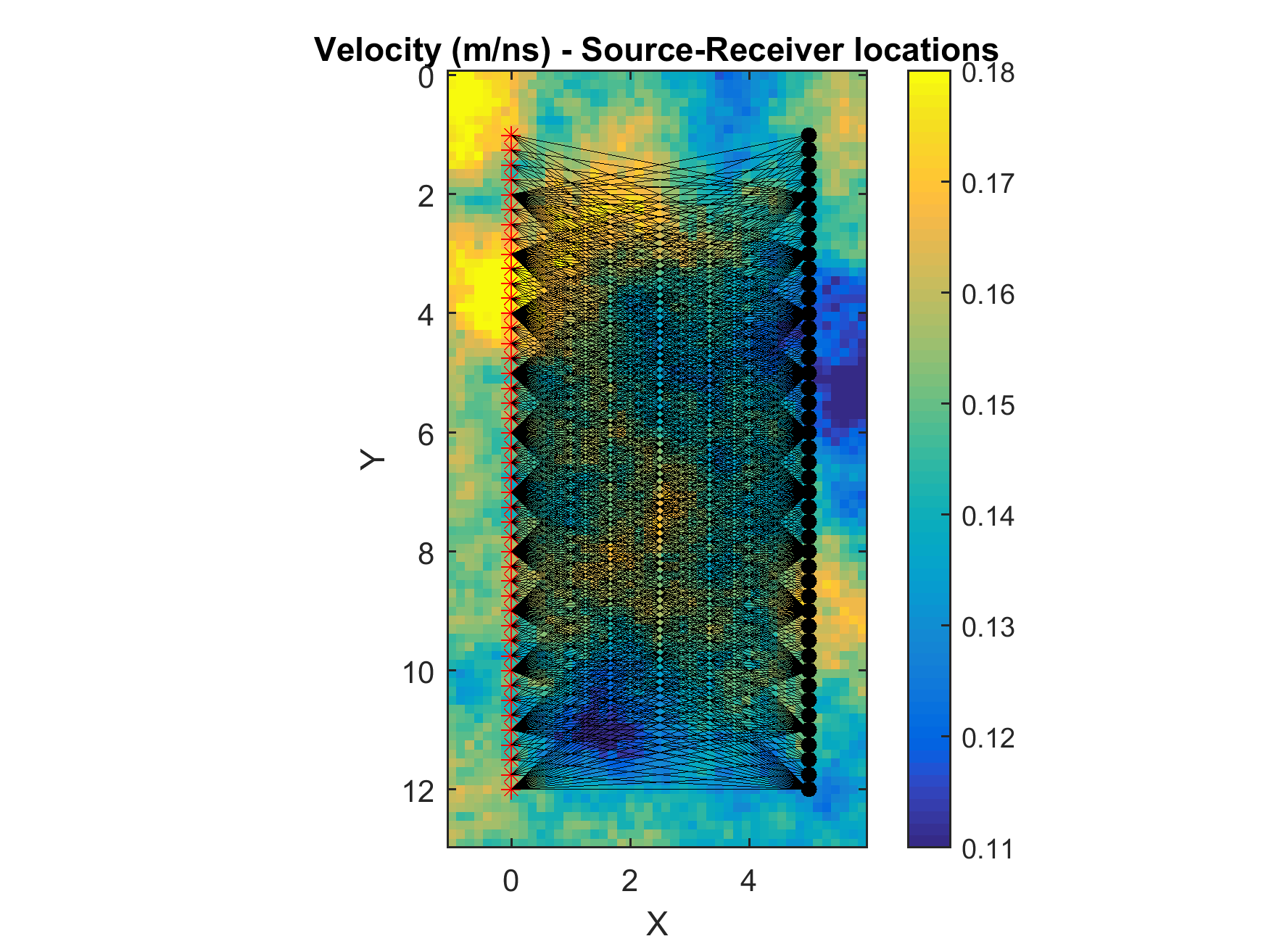
In order to visualize the Source-Receiver setup, and linear forward operator (for the linear kernels only) run the following
sippi_plot_traveltime_kernel(forward,prior);
Testing the setup
As the prior, data, and forward have been defined, one can in principle initiate an inversion. However, it is advised to perform a few test before applying the inversion.
First, one should check that independent realization of the prior model resemble the a priori knowledge. A sample from the prior model can be generated and visualized calling
sippi_plot_prior_sample
sippi_plot_prior_sample(prior);
which provides the following figure The one can check that the forward solver, and the computation of the likelihood wors as expected using
% generate a realization from the prior
m=sippi_prior(prior);
% Compute the forward response related to the realization of the prior model generated above
[d]=sippi_forward(m,forward,prior,data);
% Compute the likelihood
[logL,L,data]=sippi_likelihood(d,data);
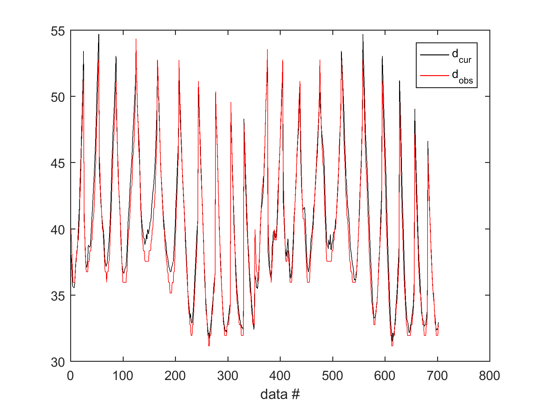
% plot the forward response and compare it to the observed data
sippi_plot_data(d,data);
which produce a figure of the forward response of a realization of the prior, compared to observed data in data{1}.d_obs:
Sampling the a posterior distribution using the extended Metropolis algorithm
The extended Metropolis sampler can now be run using sippi_metropolis.
options=sippi_metropolis(data,prior,forward);
In practice the user will have to set a few options, controlling the behavior of the algorithm. In the following example the number of iterations is set to 500000; the current model is saved to disc for every 2500 iterations. The step-lengt, data fit, log-likelihood and current model is shown for every 1000 iterations:
options.mcmc.nite=500000; % optional, default:nite=30000
options.mcmc.i_sample=2500; % optional, default:i_sample=500;
options.mcmc.i_plot=5000; % optional, default:i_plot=50;
options=sippi_metropolis(data,prior,forward,options);
By default the 'step'-length for sequential Gibbs sampling is adjusted (to obtain an average acceptance ratio of 30%) for every 50 iterations until iteration number 1000.
An output folder will be generated with a filename formatted using 'YYYYMMDD-HHMM', followed by a automatic description. In the above case the output folder could be name 20140701_1450_sippi_metropolis_eikonal. The actual folder name is returned in options.txt.
One can define a description for the folder name by setting options.txt before running sippi_metropolis.
The folder contains one mat file, with the same name as the folder name, and N ASCII files (where N=length(prior); one for each a priori type) which contains the models saved to disc. They also have the same name as the folder name, appended with '_m1.asc', '_m2.asc', and so forth.
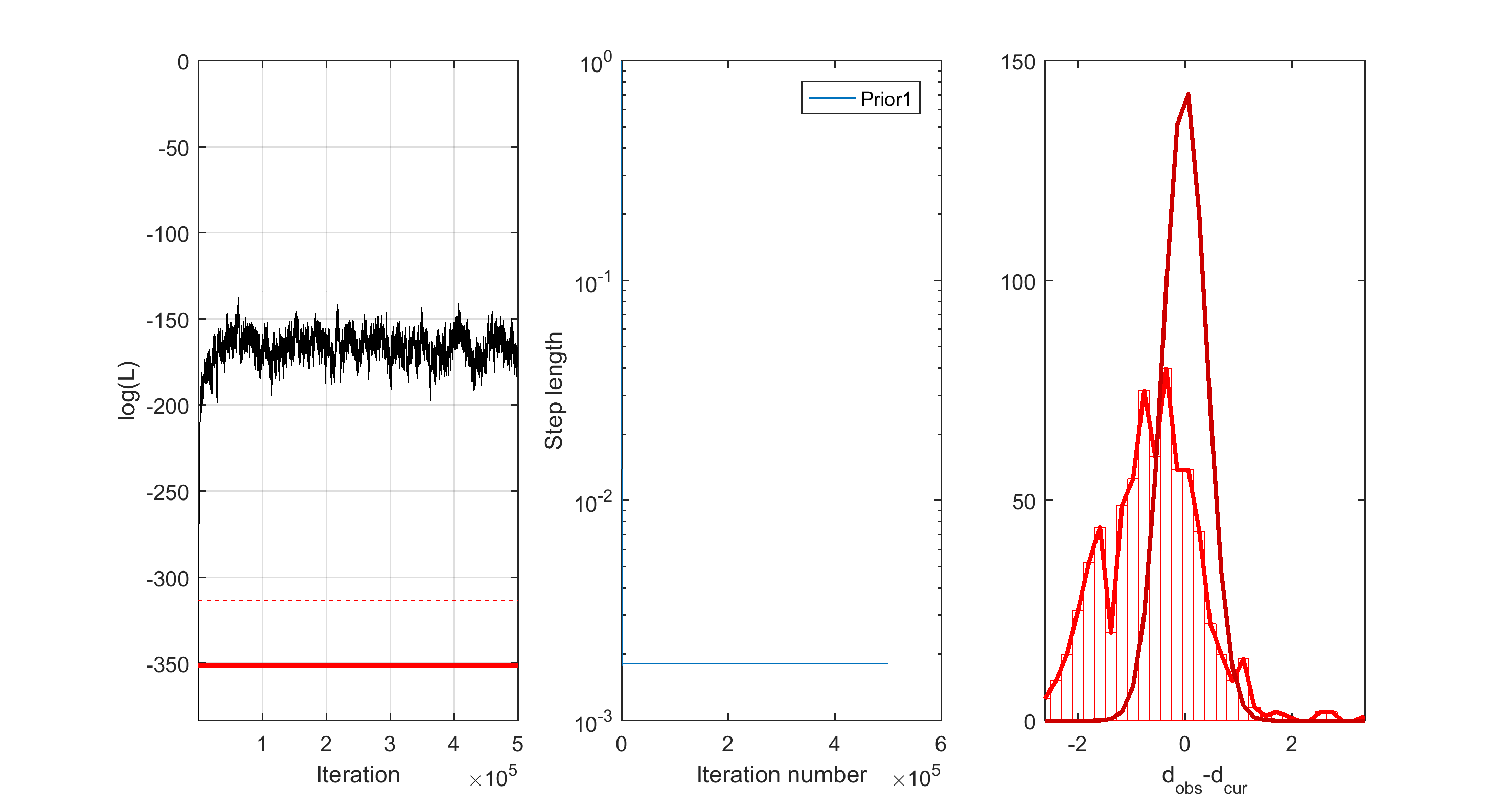
As the sampling is performed, progress the progress in likelihood, step-lengt and data mistfit is shown as e.q.
Posterior statistics
A number of plots can be generated automatically after the sampling has ended, using sippi_plot_posterior.m. One can either be located in the folder from which sippi_metropolis was run and do:
sippi_plot_posterior(options.txt);
or one can go to the folder created by sippi_metropolis and do
cd 20140701_1450_sippi_metropolis_eikonal
sippi_plot_posterior;
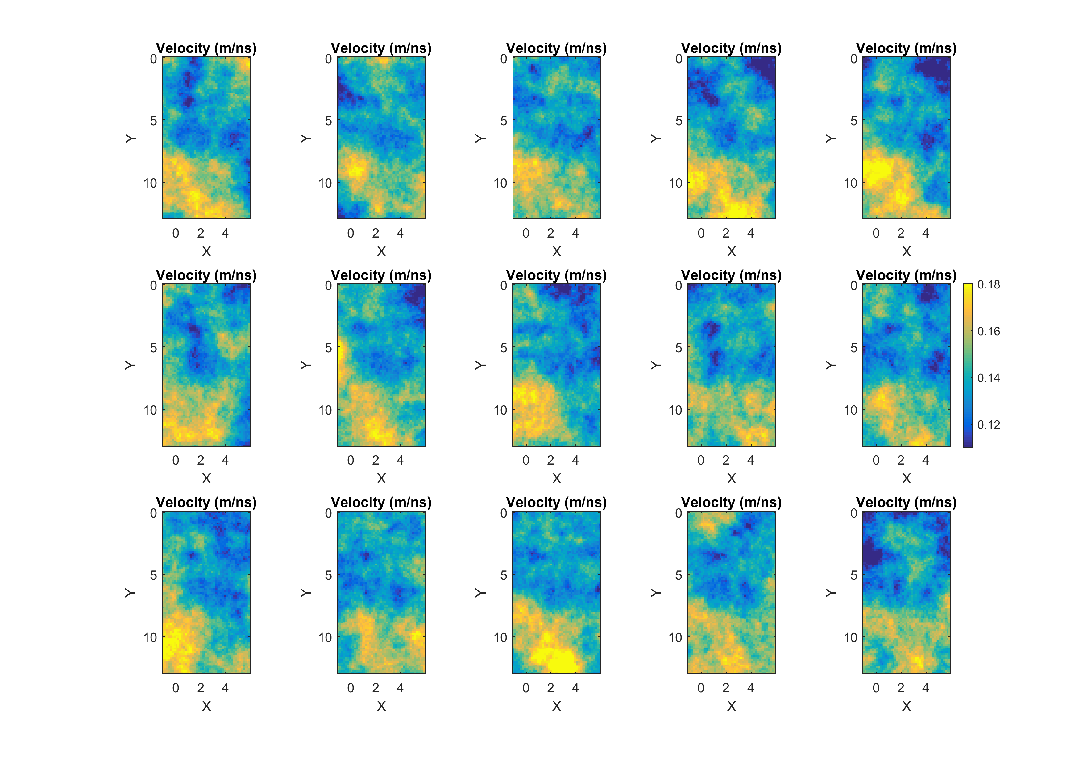
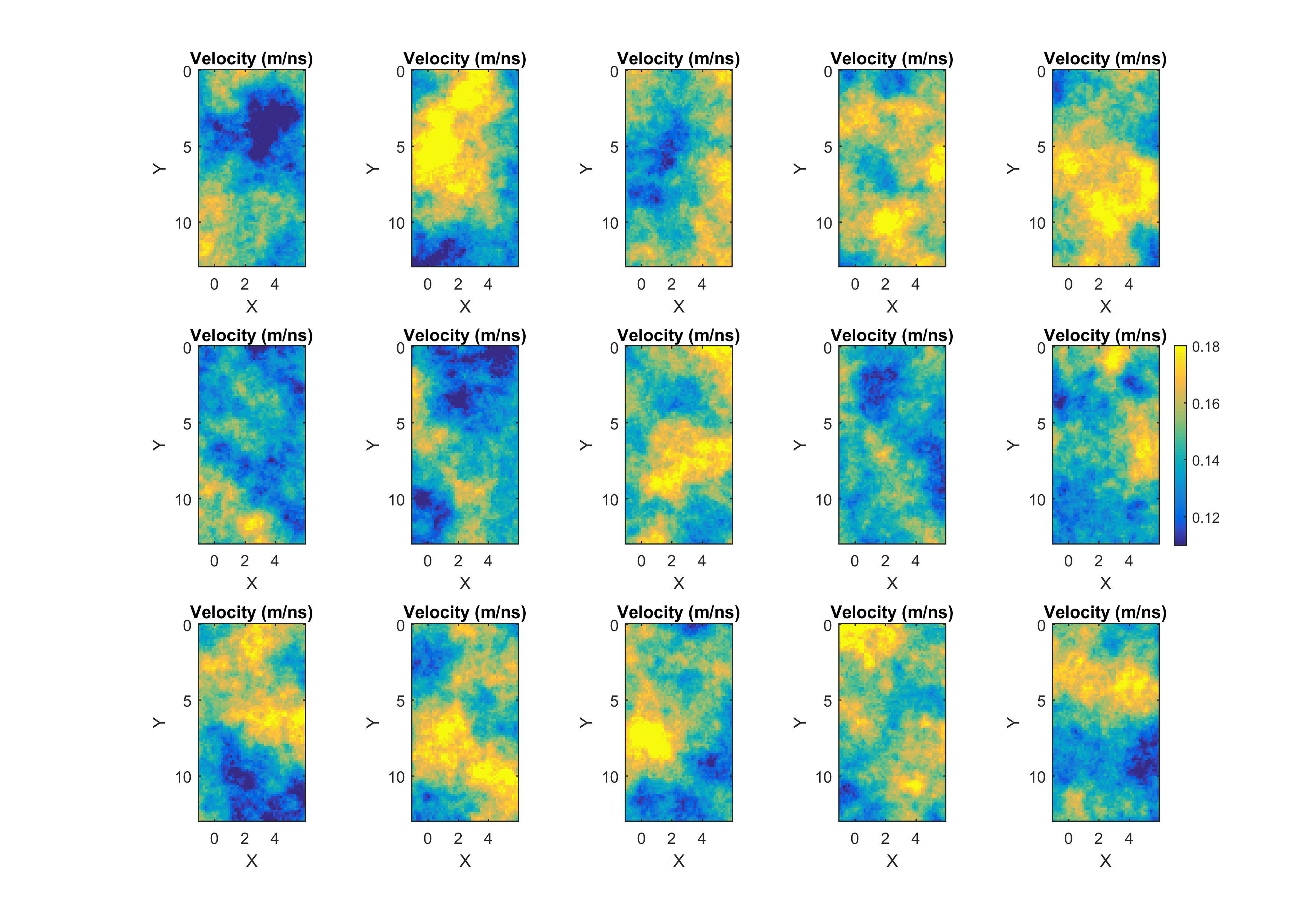
This will visualize for example a sample (consisting of 15 realizations) from the posterior:
which should be compared the a similar sample of the prior distribution:
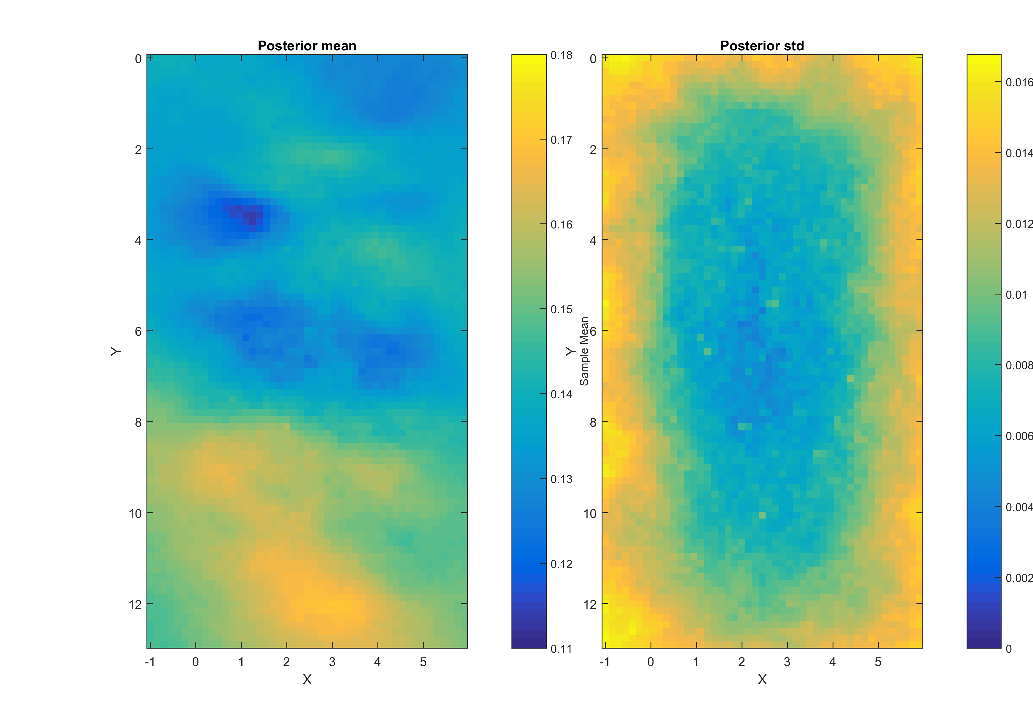
The point-wise mean and standard deviation (E-types) are also shown:
Also a movie of 200 (if that many has been created) posterior realizations is generated: